


Next: Generalized Force Balance Equations
Up: Background
Previous: Background
In the original snake formulation of Kass et al. [1], the
best snake position was defined as the solution of a variational
problem requiring the minimization of the sum of internal and external
energies integrated along the length of the snake. The corresponding
Euler equations, which give the necessary conditions for this
minimizer, comprise a force balance equation. By introducing a
temporal parameter t, the force balance equation can be made
dynamic. When the dynamic equation reaches its steady state, a
solution to the static problem is found.
We now give a brief summary of these steps.
A snake is a curve
![${\bf x}(s) = [x(s),y(s)]$](img9.gif) ,
,
![$s\in[0,1]$](img10.gif) ,
that moves through the
spatial domain of an image to minimize the energy functional
,
that moves through the
spatial domain of an image to minimize the energy functional
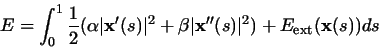 |
(1) |
where  and
and  are weighting parameters that
control the snake's tension and rigidity, respectively.
are weighting parameters that
control the snake's tension and rigidity, respectively.
 and
and
 denote the first and second derivatives of
 with respect to s. The external energy
function
with respect to s. The external energy
function
 is derived from the image so that it takes on
its smaller values at the features of interest, such as
boundaries.
is derived from the image so that it takes on
its smaller values at the features of interest, such as
boundaries.
Given a gray-level image I(x,y) (viewed as a function of continuous
position variables (x,y)), typical external energies designed to
lead an active contour toward step edges are [1]:
where
 is a two-dimensional Gaussian function with
standard deviation
is a two-dimensional Gaussian function with
standard deviation  and
and  is the gradient operator. If
the image is a line drawing (black on white), then appropriate
external energies include [20]:
is the gradient operator. If
the image is a line drawing (black on white), then appropriate
external energies include [20]:
It is easy to see from these definitions that larger 's will
cause the boundaries to become blurry. Such large 's are often
necessary, however, in order to make the effect of the boundary ``felt''
at some distance from the boundary -- i.e., to increase the capture
range of the active contour.
A snake that minimizes E must satisfy the Euler equation
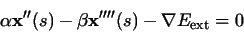 |
(6) |
This can be viewed as a force balance equation
where
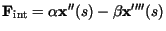 and
and
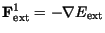 .
The
internal force
.
The
internal force
 discourages stretching and bending while
the external force
discourages stretching and bending while
the external force
 pulls the snake towards the desired image contour.
To find a solution to (6), the snake is made dynamic by
treating  as function of time t as
well as s -- i.e.,
as function of time t as
well as s -- i.e.,
 .
Then, the partial derivative of
with respect to t is then set equal to
the left hand side of (6) as follows
.
Then, the partial derivative of
with respect to t is then set equal to
the left hand side of (6) as follows
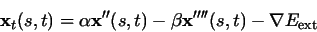 |
(7) |
When the solution
stabilizes, the term
 vanishes and we achieve a
solution of (6).
This dynamic equation can also be viewed as a gradient descent
algorithm [25] designed to solve (1).
A solution to (7) can be found by
discretizing the equation and solving the discrete system
iteratively (cf. [1]).
vanishes and we achieve a
solution of (6).
This dynamic equation can also be viewed as a gradient descent
algorithm [25] designed to solve (1).
A solution to (7) can be found by
discretizing the equation and solving the discrete system
iteratively (cf. [1]).
Next: Generalized Force Balance Equations
Up: Background
Previous: Background
Chenyang Xu
1999-11-06