Difference between revisions of "Retinal layer segmentation of macular OCT images"
(New page: <meta name="title" content="Retinal layer segmentation of macular OCT images using boundary classification"/> {{h2|Retinal layer segmentation of macular OCT images using boundary classific...) |
|||
| Line 31: | Line 31: | ||
| − | In 3D, OCT volumes comprise multiple cross-sectional images, or | + | In 3D, OCT volumes comprise multiple cross-sectional images, or ''B-Scans''. Every B-scan consists of a series of scan-lines (''A-scans'') which are in the direction of the light propagation into the tissue of interest. The inter-B-scan distance is often greater than the in-plane resolution, but this can vary by manufacturer and scanner settings. A coordinate system consisting of x,y, and z axes is created from lateral , axial, and through plane directions. |
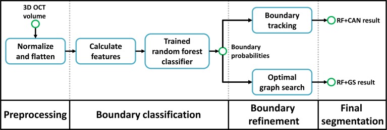
Our algorithm has three steps. The first is preprocessing the data using intensity and spatial normalization. This is followed by a set of 27 features calculated on the preprocessed data and input into a trained RF classifier to produce boundary probabilities at every pixel. In the last step, the final retina segmentations are generated from the boundary probabilities using a boundary refinement algorithm. We explore the use of two such algorithms, a simple boundary tracking method and a multi-surface graph based method, RF+CAN and RF+GS. RF+CAN is a is a 2D algorithm which operates on each B-scan independently while RF+GS operates on the whole 3D volume at once. | Our algorithm has three steps. The first is preprocessing the data using intensity and spatial normalization. This is followed by a set of 27 features calculated on the preprocessed data and input into a trained RF classifier to produce boundary probabilities at every pixel. In the last step, the final retina segmentations are generated from the boundary probabilities using a boundary refinement algorithm. We explore the use of two such algorithms, a simple boundary tracking method and a multi-surface graph based method, RF+CAN and RF+GS. RF+CAN is a is a 2D algorithm which operates on each B-scan independently while RF+GS operates on the whole 3D volume at once. | ||
Revision as of 17:24, 12 June 2014
<meta name="title" content="Retinal layer segmentation of macular OCT images using boundary classification"/>
Retinal layer segmentation of macular OCT images using boundary classification
Andrew Lang, Aron Carass, Matthew Hauser, Elias S. Sotirchos, Peter A. Calabresi, Howard S. Ying, and Jerry L. Prince
This page is under construction
Introduction
Optical coherence tomography (OCT) has proven to be an essential imaging modality for ophthalmology and is proving to be very important in neurology. OCT allows for high resolution imaging of the retina, both at the optic nerve head and the macula. Macular retinal layer thicknesses provide useful diagnostic information and have been shown to correlate well with measures of disease severity in several diseases. Since manual segmentation of these layers is time consuming and often biased, automatic segmentation methods would improve the technology significantly. In this work we build a random forest classifier to segment eight retinal layers in macular cube images acquired by OCT. The random forest classifier learns the boundary pixels between layers, producing an accurate probability map for each boundary, which is then processed to finalize the boundaries. Using this algorithm, we can accurately segment the entire retina contained in the macular cube to an accuracy of at least 4.3 microns for any of the nine boundaries.
Methods
In 3D, OCT volumes comprise multiple cross-sectional images, or B-Scans. Every B-scan consists of a series of scan-lines (A-scans) which are in the direction of the light propagation into the tissue of interest. The inter-B-scan distance is often greater than the in-plane resolution, but this can vary by manufacturer and scanner settings. A coordinate system consisting of x,y, and z axes is created from lateral , axial, and through plane directions.
Our algorithm has three steps. The first is preprocessing the data using intensity and spatial normalization. This is followed by a set of 27 features calculated on the preprocessed data and input into a trained RF classifier to produce boundary probabilities at every pixel. In the last step, the final retina segmentations are generated from the boundary probabilities using a boundary refinement algorithm. We explore the use of two such algorithms, a simple boundary tracking method and a multi-surface graph based method, RF+CAN and RF+GS. RF+CAN is a is a 2D algorithm which operates on each B-scan independently while RF+GS operates on the whole 3D volume at once.
Data from the right eyes of 35 subjects were obtained using a spectralis OCT system (Heidelberg Engineering, Heidelberg, Germany). Of the 35 subjects, 21 were diagnosed with MS while the other 14 were healthy controls. All scans were screened and found to be free of microcystic macular edema (a pathology sometimes found in MS subjects). The age range was from 20 to 56 years old.
The general properties of our RF classifier are specified by the number of trees ![]() and the number of features
and the number of features ![]() that are used at each node of each tree. The quality of training is dependent on the of subjects
that are used at each node of each tree. The quality of training is dependent on the of subjects ![]() and number of B-scans
and number of B-scans ![]() per subject. In selecting values for these parameters, we are interested in finding the set which provide a good segmentation accuracy without adding significant computational cost (as would be the case with more trees, more training data, etc.). We are not necessarily interested in finding the optimal set. To find suitable values for these parameters, we evaluated the performance of our RF classifier (using the RF+CAN algorithm) in a series of four experiments applied to 10 out of 35 subjects. We did not use the entire dataset to carry out parameter selection because of the computational burden.
per subject. In selecting values for these parameters, we are interested in finding the set which provide a good segmentation accuracy without adding significant computational cost (as would be the case with more trees, more training data, etc.). We are not necessarily interested in finding the optimal set. To find suitable values for these parameters, we evaluated the performance of our RF classifier (using the RF+CAN algorithm) in a series of four experiments applied to 10 out of 35 subjects. We did not use the entire dataset to carry out parameter selection because of the computational burden.
|
Experiment
The nine layer boundaries were manually delineated on all B-Scans for all subjects by a single rater using an internally developed protocol and software tool. The manual delineations were performed by clicking on approximately 20-50 points along each layer border followed by interpolation between the points using a cubic B-spline. Visual feedback was used to move each point to ensure a curve that correctly identifies the boundary.
In each experiment, we swept through the values of one of the four parameters while keeping the other three fixed to a reasonable value (thus generating a new set of parameters). For example, to find appropriate values for each of ![]() ,
, ![]() , and
, and ![]() , we used three training subjects (
, we used three training subjects (![]() =3). To reduce the possibility of bias from training on particular subjects , a cross-validation strategy was used whereby a set of 10 classifiers were trained for every parameter set, each trained with
=3). To reduce the possibility of bias from training on particular subjects , a cross-validation strategy was used whereby a set of 10 classifiers were trained for every parameter set, each trained with ![]() different randomly chosen subjects (from the pool of 10 subjects). For each trained classifier, we generated segmentations for the 10-
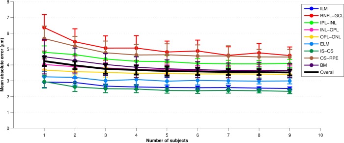
different randomly chosen subjects (from the pool of 10 subjects). For each trained classifier, we generated segmentations for the 10-![]() test subjects not used in training. The overall error for each parameter set was calculated by averaging the absolute error between the segmentation and the manual segmentation across all test subjects evaluated with each of the 10 classifiers. Figure 6 provides an example error plot for each later as the parameter
test subjects not used in training. The overall error for each parameter set was calculated by averaging the absolute error between the segmentation and the manual segmentation across all test subjects evaluated with each of the 10 classifiers. Figure 6 provides an example error plot for each later as the parameter ![]() is varied from one to nine. The error bars represent the standard deviation of the error across the 10 trials. Similar experiments were performed for the other 3 parameters. Finally, we note that for the
is varied from one to nine. The error bars represent the standard deviation of the error across the 10 trials. Similar experiments were performed for the other 3 parameters. Finally, we note that for the ![]() experiments, a separate test set of 10 subjects was used to maintain a consistent number of test subjects as
experiments, a separate test set of 10 subjects was used to maintain a consistent number of test subjects as ![]() was varied (it would not be fair to compare
was varied (it would not be fair to compare ![]() =1 with
=1 with ![]() =8 by evaluating on 10-
=8 by evaluating on 10-![]() =9 and 2 test subjects, respectively).
=9 and 2 test subjects, respectively).
|
Each of the parameters exhibited good stability and accuracy over a range of values. As a balance between performance and efficiency, we chose the ‘‘final set’’ of parameters (FSP) to be {![]() =60,
=60, ![]() =10,
=10, ![]() =7,
=7, ![]() =8}. Using values larger than these show only a small performance improvement at a much larger computational burden. With
=8}. Using values larger than these show only a small performance improvement at a much larger computational burden. With ![]() =7 and
=7 and ![]() =8, a total of 56 manual B-scan segmentations are needed for training. In an effort to reduce the amount of training data that are needed and ti reduce the loading time, computation time, and memory requirements of the classifier, we also evaluated the algorithm using a ‘‘minimal set’’ of parameters (MSP), chosen to be {
=8, a total of 56 manual B-scan segmentations are needed for training. In an effort to reduce the amount of training data that are needed and ti reduce the loading time, computation time, and memory requirements of the classifier, we also evaluated the algorithm using a ‘‘minimal set’’ of parameters (MSP), chosen to be {![]() =20,
=20, ![]() =5,
=5, ![]() =2,
=2, ![]() =4}. In this case, with
=4}. In this case, with ![]() =2 and
=2 and ![]() =4, only 8 manual B-segmentations are needed for training.
=4, only 8 manual B-segmentations are needed for training.
We evaluated our two segmentation methods, RF+CAN and RF+GS, on all 35 subjects using both the MSP and FSP. There were 10 previously trained classifiers constructed using FSP. We used the classifiers for the final evaluation of each algorithm. With the FSP, ![]() =7 randomly chosen subjects (out of a pool of 10 subjects) were used to train each of the 10 classifiers. Each classifier was evaluated by computing a segmentation on the 35-7=28 remaining test subjects.
=7 randomly chosen subjects (out of a pool of 10 subjects) were used to train each of the 10 classifiers. Each classifier was evaluated by computing a segmentation on the 35-7=28 remaining test subjects.
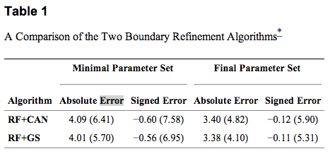
To compare the results of our algorithm against the manual delineations, we calculated the absolute and signed boundary errors for every point on every surface. These errors were then averaged over all boundaries, subjects, and cross-validation runs. Table 1 shows the results for the two different algorithms with both parameter sets. The standard deviations were calculated assuming that every error value is separate (i.e. errors were not averaged for each subject before calculation). For both algorithms, we observe significantly better performance using the FSP over the MSP (p<0.001). Significance was calculated on the average signed error over the whole volume across subjects using a one-sided paired Wilcoxon signed rank test. The MSP still performs well, however, having mean absolute errors about 0.60 μm larger than the FSP. For the same parameter set, the main difference between RF+CAN and RF+GS is that RF+GS has a lower standard deviation of error.
|
Results
The results for both of our algorithms show excellent performance with overall average absolute errors below 3.5 μm and less than 4.5 μm for any one specific boundary. Although the overall average errors are nearly identical between the two algorithms, the standard deviation of the RF+CAN algorithm is slightly larger due to the occasional possibility that the boundary tracking algorithm fails in some areas. The spatial smoothness constraints imposed by the graph search algorithm prevent these failures in the RF+GS algorithm. Looking at the thickness values calculated using RF+GS algorithm, we see average errors of less than 3 μm in 81% of the sectors and standard deviation values less than 3 μm in 90% of the sectors indicating a high level of confidence in these measurements. When using the minimal training set, the errors are larger but the performance is still quite good, with errors only slightly larger than the axial resolution of the system. Therefore, training the RF from a new data source-i.e., for a new system or for new parameters on an existing system-could be carried out within only a few hours in order to achieve adequate performance when using the minimal training set. When comparing our algorithm with other retinal segmentation methods found in the literature, we see comparable performance to the best algorithms [Q. Yang et. al., S.J. Chiu et. al., P.A. Dufour et. al.], each of which shows average errors of between 3-4 μm. This comparison is inherently difficult, however, as the methods are evaluated on data acquired with different types f scanners using different numbers of manually delineated subjects (as few as 10 subjects). Due to the time consuming nature of manual segmentation, evaluations are often performed against only a subset of the full data (5-10 B-scans per subject), which includes many poor quality images. Our manual segmentations are also generated as smooth spline curves from a small set of control points, which is different from other manual delineations and thus may introduce bias.
Looking to the future, although the algorithm performance was not degraded for MS subjects, we expect that modifications will be necessary to handle other pathologies such as microcysts, drusen, and geographic atrophy (GA). There are many possible solutions for modification of our algorithm to handle these retinal pathologies. One possible approach for handling microcysts and drusen is by a pre-classification of the pathological areas. These areas could then be incorporated into the spatial features enabling the random forest classifier to learn an alternate model in these regions. In the case of partially or completely missing layers, it may be necessary to remove the spatial features from these areas and rely on intensity features to guide the final segmentation. A pre-idetification of the ILM and BrM would still prove to be invaluable to the segmentation as additional constraints on the graph algorithm can be incorporated to handle these cases [P.A. Dufour et. al.].
In the case of structurally normal eyes, there are still several potential areas of improvement-for example, allowing the RF to know if an A-scan has a blood vessel shadow could improve our results. We have a good idea of which regions and layers are more difficult to segment allowing us to focus on finding improvements for these areas. With regards to the graph-based segmentation in the second part of our work, learning boundary specific constraints at each surface position would improve the segmentation and further help to eliminate outliers in the final segmentation.
Acknowledgements
This work was supported by the NIH/NEI under grant R21-EY022150
Publications
- A. Lang, A. Carass, M. Hauser, E. S. Sotirchos, P.A. Calabresi, H.S. Ying, and J.L. Prince, "Retinal layer segmentation of macular OCT images using boundary classification", Biomedical Optics Express, 4(7):1133-1152, 2013.

- A.Lang, A. Carass, E.S. Sotirchos, P.A. Calabresi, and J.L. Prince, "Segmentation of retinal OCT images using a random forest classifier", Proceedings of SPIE Medical Imaging (SPIE-MI 2013), Orlando, FL, February 9-14, 2013. (PubMed)
- A. Carass, A. Lang, M. Hauser, P.A. Calabresi, H.S. Ying, and J.L. Prince, "Multiple-object geometric deformable model for segmentation of macular OCT", Biomedical Optics Express, 5(4):1062-1074, 2014.

References
- Q. Yang, C.A. Reisman, Z. Wang, Y. Fukuma, M. Hangai, N. Yoshimura, A. Tomidokoro, M. Araie, A.S. Raza, D.C. Hood, and K. Chan, "Automated layer segmentation of macular OCT images using dual-scale gradient information", Optics Express, 18(20):21293-21307, 2010.


