MR Image Synthesis by Contrast Learning On Neighborhood Ensembles

<meta name="title" content="MR Image Synthesis by Contrast Learning on Neighborhood Ensembles"/>

MR Image Synthesis by Contrast Learning On Neighborhood Ensembles

Amod Jog, Aaron Carass, Snehashis Roy, Dzung L. Pham, and Jerry L Prince

Introduction

Automatic processing of magnetic resonance images is a vital part of neuroscience research. Yet even the best and most widely used medical image processing methods will not produce consistent results when their input images are acquired with different pulse sequences. Although intensity standardization and image synthesis methods have been introduced to address this problem, each method has their own shortcomings. In this paper, we improve upon these approaches by using atlas-based intensity transformation ideas while incorporating the MR image formation process.

A previous work by Amod Jog (Magnetic resonance image synthesis through patch regression) presented a patch-based regression approach using random forest regression for synthesizing MR images. While the method presented was extremely quick, it required the subject image to be intensity standardized to the atlas image prior to applying the learned regression ad does not account for MR physics of acquisition. In this paper we build upon this random forest regression by synthesizing a new subject image from the available subject image(s) and a set of atlas images. While the core idea of estimating tissue parameters was used in previous work (Fischel et. al. 2004), the previous approach required the acquisition of very specific pulse sequences while our new approach does not require that information. We call our new method “Pulse Sequence Information-based Contrast Learning On Neighborhood Ensembles” (PSI-Clone) which we stylize as Ψ-CLONE.

Method

Figure 1: A flow chart of the Ψ-CLONE algorithm.

The first step of Ψ-CLONE estimates the imaging parameters from the subject image. Let 𝔹= {b₁, b₂,..., b_m} be the given subject image set imaged with pulse sequences Γ₁, . . . , Γ_m. This set can contain images from different pulse sequences such as MPRAGE, spoiled gradient recalled (SPGR) and DSE. Also, let 𝔸= {a₁, a₂,..., a_n} be the atlas collection with images of contrasts 𝑪₁,..., 𝑪_n, generated by pulse sequences Ψ₁,..., Ψ_n, respectively. By pulse sequences we mean paticular, name procedures like MPRAGE. By contrast we mean the tissue contrast produced by a pulse sequence, say a T₁-weighted contrast or a T₂-weighted contrast. For instance, the MPRAGE pulse sequence produces a T₁-w contrast image. Since in most cases our data consists of specific pulse sequences producing specific contrasts, these terms can be used interchangeably.

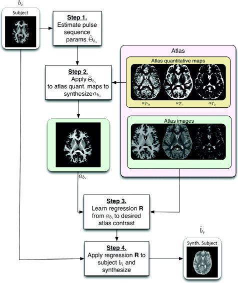
The pulse sequence sets Γ₁, . . . , Γm and Ψ₁,..., Ψ_n do not need to intersect which is an important distinction between Ψ-CLONE and other atlas-based image synthesis methods. Our goal is to synthesize the image , r ∈ { P t₁ . . . , n}, which is how the subject brain would look had it been imaged with pulse sequence Ψ_r used to acquire the atlas image ar. The first step of the algorithm is to estimate the the pulse sequence parameters used to acquire b_i, i∈ {1,...,m}. The second step of the algorithm aims to generate a_bi the atlas image with the same contrast, 𝑪_i, as b_i using the the estimate from the first part of the algorithm. The third step of the algorithm uses the expanded atlas collection 𝔸∪{a_bi} and with that we learn the nonlinear intensity transformation between contrast 𝑪_i and the target contrast image a_r. The final and fourth step of the algorithm is that the intensity transformation is applied to b_i, generating the subject image , of the desired contrast. These steps are outlined in Figure 1 as a flow chart.

Results

Completed tests with two different sets of data, one set of phantom data and one set of real data.

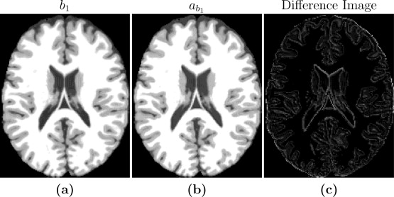
For our initial phantom tests, the goal was to produce synthetic images that are useful substitutes for real images for image processing tasks. Thus, one aspect of algorithm performance evaluation consists of using image quality metrics to compare synthetic images with known ground truth images. The controlled setting allows us to compare our synthetic images with the know simulated images to validate our method in a controlled setting. We went through the steps with the phantom data, the first step being estimating the imaging parameters. When this is done we moved to step two in which we create a synthetic atlas image using the pulse sequence parameters of the subject image. Since the anatomy of subject and atlas is the same in this special case, we can directly compare the synthetic atlas image with the subject image to validate if the pulse sequence parameters with the are producing an identical image. Figure 2 shows the input b₁, the estimated b₁ image as well as a difference image for the case of a=45*. The images are very similar to each other with small differences at tissue boundaries. The reason for the differences at the boundaries is because Brainweb phantom images (the ones used for the test) with no noise typically have very homogenous intensity distribution in each of the tissue classes (WM, GM, CSF). Hence the error inside the tissues is very close to zero, but is slightly higher at the intermediate intensity voxels that are closer to the boundaries. But the results from these tests confirm that the theoretical pulse sequence equations and the underlying quantitative PDT₁ and T₂ maps produce images that are close to the ground truth images, thus validating the first two steps of our algorithm. The experiment we conducted to test the validity of steps three and four is an experiment with the goal to standardize a Brainweb SPGR subject image to an atlas SPGR image. Different subject images were simulated using different input pulse sequence parameters. Using the Brainweb atlas collection, we evaluated the results of steps three and four. We used different images with varying amounts of noise and compared our results to that of UPL. While the UPL was more accurate during 0% noise cases, in four out of five cases, our method performed better when noise was introduced to the images.

Figure 2: Shown are (a) an SPGR image (TR= 18ms, TE=10 ms, α “ 45˝ with 0% additive noise) which we use as our subject image bi, the maximum intensity value is 1080, the (b) new atlas image, ab1, with pulse sequence parameters estimated from b1, and (c) the difference image |ab1-b1|, the maximum value is 5

Figure 3: The brown plot illustrates relative WM volumes (with respect to the ICV) over nine weeks before any standardization while the green plot illustrates the same values after intensity standardization using Ψ-CLONE

For our real subject data experiments we imaged a normal, healthy human at weekly intervals using the same scanner and pulse sequence for nine weeks. Ideally, over the course of nine weeks a healthy human subject should not present any changes in tissue volumes. In order to show that image segmentation is more consistent on data which is intensity standardized using Ψ-CLONE, we standardized each time point to an atlas consisting of:

-a₁: MPRAGE image (3T, TR=10.3 ms, TE=6 ms, 0.82 x 0.82 x 1.17 mm³ voxel size)

-a_T1: Quantitative T₁ map

-a_T2: Quantitative T₂ map

-a_PD: Quantitative P_D map

and each of the nine subject images is:

-b₁: MPRAGE image (3 T, TR=10.3 ms, TE=6 ms, 0.82 x 0.82 x 1.17 mm³ voxel size) (parameters, excepting TR, not provided to the algorithm)

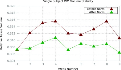
We compare the segmentations of the images pre- and post-standardization using Ψ-CLONE, based on segmentations generated by TOADS (Bazin and Pham, 2007). We specifically compare the relative tissue volumes (relative to the intra-cranial volume (ICV)), over the nine weeks. Figure 3 shows the relative WM volumes before and after Ψ-CLONE was applied. Visually, it is apparent that the WM volumes change less when standardized images are segmented. The coefficients of variation from segmentation after standardization by Ψ-CLONE are smaller than those without standardization for cortical WM, cortical and subcortical GM, and ventricles, indicating that the segmentation is more stable.

To bring in more data, we did 57 scans of 15 multiple Sclerosis patients with each subject being scanned at least three times. For this experiment our atlas consisted of:

- a₁: MPRAGE image (3T, TR=10.3ms, TE=6ms, 0.82 x 0.82 x 1.17mm³ voxel size)

-a₂: T₂-w image from the second echo of a DSE (3T, TR=4177 ms, 1TE=12.31ms, 2TE=80ms, 0.82x 0.82 x 2.2mm³ voxel size)

-a3: P_D-w from first echo of a DSE (3T, TR=4177ms, TE₁=12.31ms, TE₂=8- ms, 0.82 x 0.82 x 2.2mm³ voxel size)

-a4: FLAIR (3T, T1=11000 ms, TE=68 ms, 0.82 x 0.82 x 2.2mm³ voxel size)

-a_T1: Quantitative T₁ map -a_T2: Quantitative T₂ map

-a_PD: Quantitative PD map

and our subject was

- b₁: MPRAGE image (3T, TR=10.3 ms, Te=6 ms, 0.82 x 0.82 x 1.17mm₃ voxel size). (Parameters, excepting TR, not provided to the algorithm).

We use an atlas MPRAGE as the target pulse sequence to which we standardize the 57 data sets. We treat each data set independently, handling the intensity standardization as a cross-sectional task. We then validate the intensity standardization and segment the original datasets giving us ten labeled structures: ventricles, sulcal CSF, cerebellar GM, cortical GM, thalamus, putamen, cerebellar WM, cortical WM, and lesions. Using these structures as reference, we compared the mean intensity within these structures prior to standardization and after standardization with UPL—using the MPRAGE in our atlas as a standardization target—and our method (Ψ-CLONE). Results of this are shown in table 7 and it shows that Ψ-CLONE moves the MS data intensities closer to the atlas intensities, as desired by standardization.

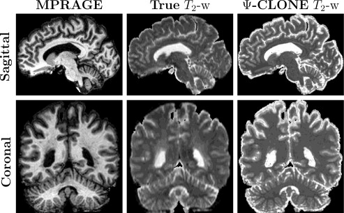
We also conducted further synthesis applications to demonstrate more potential uses for Ψ-CLONE including synthesizing higher resolution T₂-w data and FLAIR synthesis (FLAIR is the pulse sequence of choice when identifying white matter lesions present in MS patients). Figure 4 shows results of Ψ-CLONE synthesizing higher resolution T₂-w data and Figure 5 shows the results of Ψ-CLONE synthesizing a FLAIR image that originally had artifacts.

Figure 4: The MPRAGE has a through-plane resolution of 1.1~mm, while the original T2-w has through-plane resolution of 2.2~mm. This is evident as the true interpolated T2-w image shows blurring while the Ψ-CLONE synthesized image is crisp.

Figure 5: Input T1-w, T2-w images followed by the synthetic FLAIR and true FLAIR. The true FLAIR shows motion artifacts, which are not present in the synthetic FLAIR.

Conclusion

In summary, we have described a new MR synthesis approach which incorporates principles based on the pulse sequence equations. The framework is validated on synthetic and real data demonstrating its superior synthesis to state-of-the-art approaches. We have also demonstrated the capability to synthesize the FLAIR pulse sequence. Our estimation of pulse sequence parameters to generate a better atlas image could be used by any synthesis approach.

Acknowledgments

This work was supported by the NIH/NIBIB under grant R21 EB012765 and RO1 Eb017743, and by the NIH/NINDS through grant R01 NS070906.

References

• B. Fischl, D.H. Salat, A.J.W. van der kouwe, N. Makris, F. Segonne, B.T. Quinn, and A.M. Dale. Sequence-independent segmentation of magnetic resonance images. NeuroImage. 23(S1): 69-84, 2004.