 The steady-state solution (as
Equations (11a) and (11b) can be solved by
treating u and v as functions of time and solving
 The steady-state solution (as
![]() )
of these
linear parabolic equations is the desired solution of the Euler
equations (11a) and (11b). Note that these
equations are decoupled, and therefore can be solved as separate
scalar partial differential equations in u and v.
The equations in (12) are known as generalized
diffusion equations, and are known to arise in such diverse fields
as heat conduction, reactor physics, and fluid flow [30].
For us, they have
appeared from our description of desirable properties of external fields
for active contours. Diffusion is a natural outcome given the desired
``filling in'' property.
)
of these
linear parabolic equations is the desired solution of the Euler
equations (11a) and (11b). Note that these
equations are decoupled, and therefore can be solved as separate
scalar partial differential equations in u and v.
The equations in (12) are known as generalized
diffusion equations, and are known to arise in such diverse fields
as heat conduction, reactor physics, and fluid flow [30].
For us, they have
appeared from our description of desirable properties of external fields
for active contours. Diffusion is a natural outcome given the desired
``filling in'' property.
For convenience, we rewrite Equation (12) as follows
 where
where

To set up the iterative solution, let the indices i, j, and
n correspond to x, y, and t, respectively, and let the spacing
between pixels be ![]() and
and ![]() and the time step for each
iteration be
and the time step for each
iteration be ![]() .
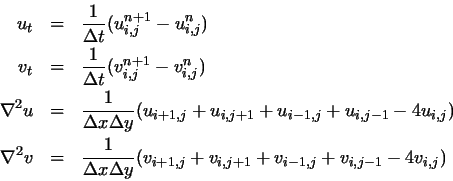
Then the required partial derivatives can be
approximated as
.
Then the required partial derivatives can be
approximated as

 where
where
Convergence of the above iterative process is guaranteed by a standard
result in the theory of numerical methods (cf. [32]). Provided
that b, c1, and c2 are bounded, (14) is
stable whenever the Courant-Friedrichs-Lewy step-size restriction
![]() is maintained. Since normally
is maintained. Since normally ![]() ,
,
![]() ,
and
,
and
![]() are fixed, using the definition of r in (15) we find
that the following restriction on the time-step
are fixed, using the definition of r in (15) we find
that the following restriction on the time-step ![]() must be
maintained in order to guarantee convergence of GVF:
must be
maintained in order to guarantee convergence of GVF: